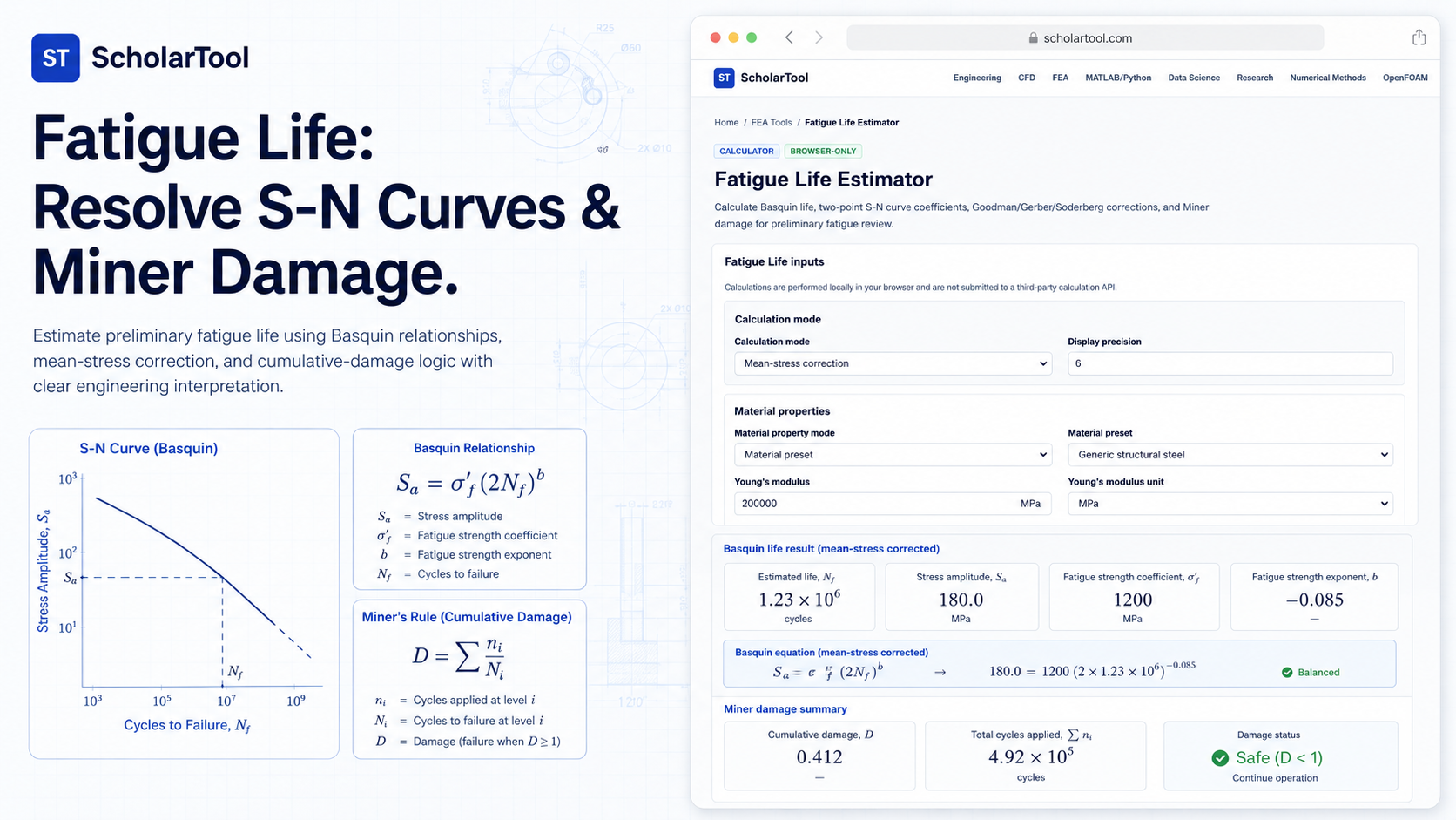
Fatigue Life Estimator: S-N Curve & Miner Damage Tool
When I am auditing a structural design, a successful static yielding check is rarely the end of the story. A component might survive its peak Von Mises demand during a single load cycle, but if that load repeats thousands of times, the material will eventually succumb to fatigue. In professional engineering, ignoring cyclical failure is a risk that leads to unexpected field failures. As Dominique Madier emphasizes in FEA Academy’s guidelines for good modeling practices, documenting mathematical checks and performing preliminary estimations are essential steps for verifying any model’s validity.
What I find indispensable for these cyclical audits is the Fatigue Life Estimator from ScholarTool. It is a deterministic, browser-local utility designed to apply stress-life (S-N) principles to preliminary design reviews. Whether I am grounding a complex FEA simulation or performing a “hand-check” for a research paper, this tool ensures my endurance assumptions are mathematically sound while keeping my proprietary project data private.
What the Fatigue Life Estimator Helps You Do
In technical terms, this tool identifies the remaining life of a component subjected to fluctuating loads. The primary purpose of the estimator is to bridge the gap between raw stress amplitudes and actionable failure predictions. I find the interface particularly useful because it allows me to move beyond simple “pass/fail” static criteria to calculate the actual number of cycles to failure.
As I have observed in textbooks like Shigley’s Mechanical Engineering Design, fatigue life is highly sensitive to mean stresses and stress concentrations. The ScholarTool interface removes the risk of manual transcription errors by providing a “browser-only” calculation engine. Because the math happens locally on your device, your sensitive manufacturing specs or proprietary load blocks are never submitted to a third-party API a critical security requirement for professional technical documentation.
Inputs You Can Use
The interface is built with a logical, “calculation-mode” layout that allows you to configure the tool based on the fatigue data you have available.
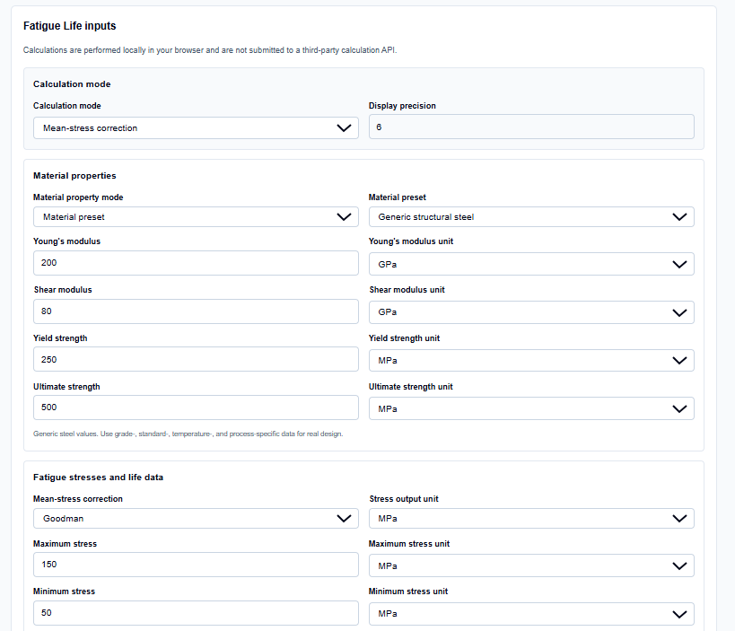
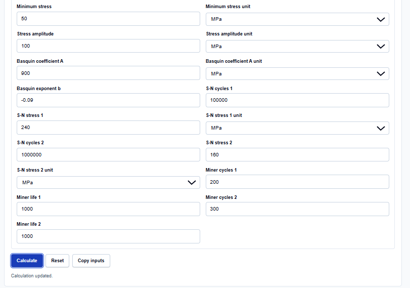
Calculation Modes
I start by selecting the mode that matches my current task:
- Basquin life: Resolves the power-law relationship between stress amplitude and life ($N$).
- Two-point S-N fit: Allows me to derive S-N curve coefficients if I only have experimental data points.
- Mean-stress correction: Essential when the stress cycle isn’t fully reversed (i.e., when there is a non-zero mean stress).
- Miner damage: Used for cumulative damage analysis when the component faces multiple different load blocks.
Material and Property Modes
You can choose from Material presets for generic steel, aluminum, or copper, or enter manual properties for proprietary alloys. What I find helpful is that the tool supports both SI (MPa) and Imperial (ksi) units, normalizing them internally to ensure consistent Basquin derivations.
A Comparative Perspective: Mean Stress Corrections
From a comparative perspective, one of the most useful features of this tool is the Mean-stress correction selection. In my experience, choosing the right theory is a matter of professional judgment. You can select:
- Goodman: The industry-standard linear approach, often used for conservative audits.
- Gerber: A parabolic model that is typically more accurate for ductile materials but less conservative.
- Soderberg: The most conservative option, as it stays below the yield line.
The tool allows you to toggle between these models to see how the “Corrected equivalent amplitude” shifts, providing the comparative context needed to justify your safety factors.
How I Use the Tool
My typical workflow begins by extracting stress probes from my FEA postprocessor or a Shaft Design Calculator. For instance, if I have a shaft with a mean stress of 50 MPa and an alternating stress of 100 MPa, I select the “Mean-stress correction” mode.
Once I enter my material’s yield and tensile strength, I click calculate. I appreciate the transparency of the Calculation steps section. It explicitly shows the formula substitutions, acting as a “math receipt” that I can archive. Because the calculations are performed locally in TypeScript, I can perform these audits during high-stakes design sessions without fear of data leakage. After the check, I use the Print summary feature to include the results directly in my technical report.
Understanding the Results
The result section provides the Basquin life or Miner damage prominently at the top. However, for a professional audit, the secondary results are often more critical:
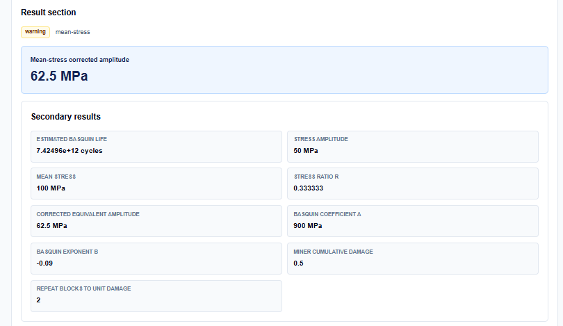
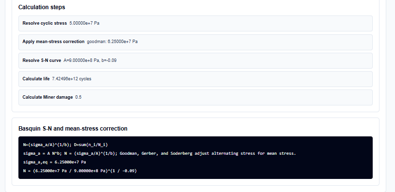
- Corrected equivalent amplitude: The effective stress used to enter the S-N curve.
- Alternating and Mean stress: A verification of the input cycle.
- Formula substitution: A transparent look at how the tool resolved the theory.
I find the Engineering interpretation indispensable. It serves as a constant reminder that these results are for educational estimation and preliminary support, not a replacement for code-compliant physical testing.
A Practical Example
Suppose I am verifying a steel component ($S_y = 250$ MPa) subjected to a constant amplitude load where the alternating stress is 150 MPa. I enter these values into the “Basquin life” mode.
The tool applies the power-law coefficients and returns the predicted number of cycles to failure. If I then determine that the component will face a second load block at 200 MPa, I switch to the “Miner damage” mode. The tool then sums the damage ($D = \sum n_i/N_i$) to see if the total exceeds 1.0, signaling failure.
Mistakes I Would Avoid
One common pitfall is using peak stress where alternating stress is required. Fatigue is driven by the range of stress, not just the maximum value.
Another mistake is ignoring stress concentrations. As the tool’s limitations remind us, it does not include automatic notch corrections. I always ensure that I enter a corrected local stress amplitude when concentration effects from keyways or fillets are present.
Try the Free Fatigue Life Estimator
Before you finalize your next structural report or sign off on a machine element, take a minute to verify your cyclical margins. It is the fastest way to ground your life-expectancy claims in physical reality.
Try the Fatigue Life Estimator here.
To complete your failure analysis, you may also find the Von Mises Stress Calculator, Shaft Design Calculator, or Factor of Safety Calculator essential for your workflow.
FAQ
1. What is the difference between Goodman and Gerber mean stress corrections?
Goodman is a linear relationship and is generally more conservative for ductile materials. Gerber uses a parabolic relationship, which often more closely matches experimental data for ductile metals but provides less of a safety margin.
2. Can this tool handle rainflow counting for complex load histories?
No. As noted in the tool’s limitations, it is intended for simple load blocks and does not perform rainflow counting for random or non-repeating stress histories.
3. Is my proprietary project data safe when using this tool?
Yes. All calculations are performed locally in your browser using TypeScript. Your inputs and results are never submitted to a third-party server or calculation API.