
Turbulence Intensity Calculator: CFD Inlet Boundary Conditions
When I am setting up a Computational Fluid Dynamics (CFD) simulation, I often find that the most daunting part isn’t the mesh or the solver settings it’s the boundary conditions. Specifically, defining how “chaotic” the fluid is as it enters the domain can determine whether a simulation converges or produces non-physical “wiggles” near the inlet. If you have ever had a $k-\epsilon$ or $k-\omega$ model fail to stabilize, you likely know the frustration of an improperly defined turbulence intensity ($I$).
What I find useful for solving this is the Turbulence Intensity Calculator from ScholarTool. It provides a deterministic, browser-local way to calculate the percentage of turbulence in your flow. Whether you are using an empirical correlation for a fully developed pipe flow or reverse-calculating intensity from experimental probe data, this tool ensures your simulation starts on solid ground.
What Turbulence Intensity Is and Why It Matters
In technical terms, turbulence intensity represents the level of velocity fluctuations relative to the mean flow. As noted in the Elements of Computational Fluid Dynamics, turbulence is essentially a highly disorganized state of flow where vortices of various scales are superimposed on the main flow. The intensity is the ratio of the Root Mean Square (RMS) of these velocity fluctuations ($u’_{rms}$) to the mean velocity ($U$).
Why is this accuracy critical? In civil engineering and aerodynamics, different flow regimes exhibit vastly different mixing and energy dissipation characteristics. For instance, a submerged jet expands rapidly because of turbulent mixing, which redistributes longitudinal velocity. If you use a “default” intensity that doesn’t match your Reynolds number ($Re$), your solver may over-predict or under-predict the rate at which these vortices dissipate energy.
A Comparative Perspective on Inlet Definitions
Many practitioners fall into the trap of using a universal “rule of thumb,” such as 5% turbulence intensity, for every simulation. However, from a comparative perspective, this is often inaccurate.
When I compare high-Reynolds-number pipe flow to low-intensity wind tunnel environments, the physical reality is quite different. In a smooth pipe at a high $Re$, the intensity might actually be closer to 3%. Conversely, in the wake of complex machinery, it could exceed 10%. Using the calculator allows you to move beyond generic guesses and ground your boundary conditions in established empirical correlations or direct experimental data.
Inputs You Can Use
The interface is designed with a clear “config-first” logic. I have noticed that it processes everything locally in your browser, which is a major advantage when you are working with proprietary industrial flow parameters that cannot be uploaded to a third-party API.
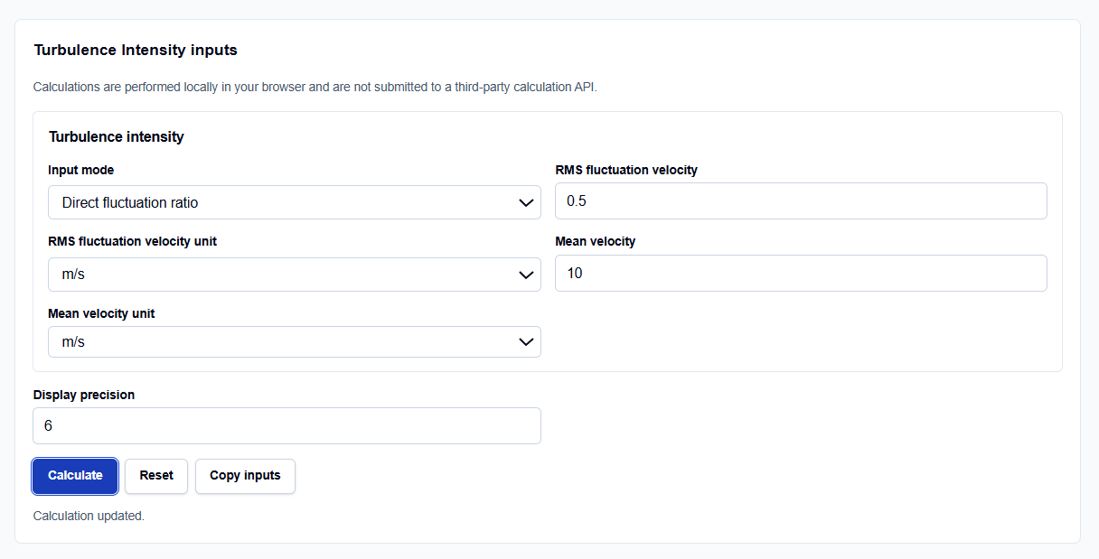
1. Direct Mode (Fluctuation Data)
If you have experimental data from a Hot-Wire Anemometer or PIV (Particle Image Velocimetry), you can use the Direct mode. You enter the RMS velocity fluctuation ($u’{rms}$) and the Mean velocity ($U$). The tool then solves the fundamental definition: $I = u’{rms} / U$.
2. Reynolds Estimate (Empirical Mode)
If you are simulating internal pipe or duct flow and only know your flow regime, select the Reynolds estimate. It uses a well-accepted empirical power-law correlation: $$I = 0.16 \cdot Re^{-1/8}$$ I find this particularly helpful because it accounts for the fact that as the Reynolds number increases, the relative intensity of turbulence tends to decrease, even as the absolute fluctuations grow.
3. Preset Mode
For preliminary reviews where exact data is missing, the Preset mode provides example inlet levels (Low, Medium, High) to help you understand typical CFD contexts.
How I Use the Tool
My workflow typically starts with the Reynolds Number Calculator to define my flow regime. Once I have my $Re$, I open the Turbulence Intensity interface.
When you enter your values, you can choose various units; the calculator internally normalizes these to SI. I appreciate that the results remain hidden until you click the Calculate action button, which ensures you have reviewed your inputs—like ensuring you haven’t confused RMS fluctuation with mean velocity.
Understanding the Results
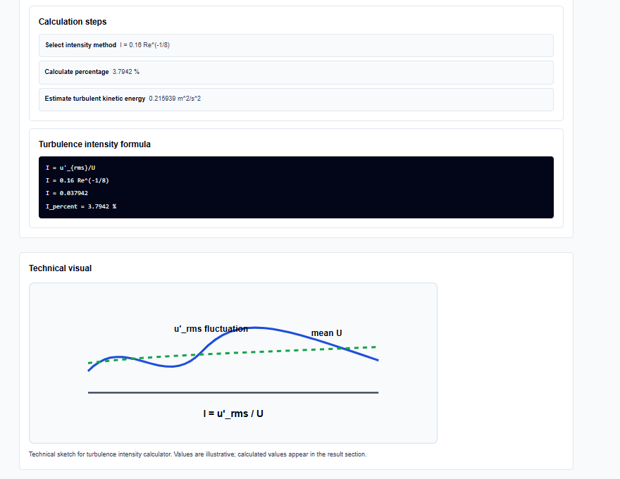
The primary result is the Turbulence Intensity ($I$) expressed as both a decimal and a percentage. What I find most valuable for solver setup is the Isotropic turbulent kinetic energy ($k$) estimate. This derived value, calculated as $k = 3/2(UI)^2$, is often required as a direct input for $k-\epsilon$ turbulence models.

The tool also provides an Engineering interpretation, reminding you to check your solver-model requirements before using the value. It’s a “sanity check” to ensure your boundary layer physics are grounded in reality.
A Practical Example
Suppose I am simulating water flow through a pipe at a Reynolds number of 100,000. I select the “Reynolds estimate” mode and enter 100000.
When I click calculate, the tool applies the empirical formula and returns a turbulence intensity of approximately 3.79%. If I also provide a mean velocity of 10 m/s, the tool estimates the isotropic turbulent kinetic energy at 0.216 m²/s² (based on the derived $I$). This specific value is far more precise than a generic 5% guess and provides better convergence for my solver.
Mistakes I Would Avoid
One common pitfall is using the empirical Reynolds estimate for every inlet. This formula is specifically for internal, fully developed pipe flow. For external aerodynamics—like flow over an airfoil—the turbulence is often determined by atmospheric “ambient” conditions, and the pipe correlation will not be physically valid.
Another mistake is ignoring the isotropic assumption for TKE. The $k$ estimate assumes that velocity fluctuations are the same in all directions. If your flow is highly anisotropic (like a very thin boundary layer), you should use the TKE value only as a preliminary estimate.
Try the Free Turbulence Intensity Calculator
Before you initialize your next solver run, take a minute to ground your boundary conditions in verified math. It is the fastest way to improve convergence and ensure your results match physical expectations.
Try the Turbulence Intensity Calculator here. For a complete setup review, you may also want to use the Reynolds Number Calculator to define your flow regime or the Y Plus Calculator to ensure your mesh is appropriate for the turbulence levels you have just calculated.
FAQ
1. Is 5% a good default for all CFD inlets?
No. While 5% is a common “rule of thumb” for medium-intensity industrial flows, it is often inaccurate. For example, in high-Reynolds-number smooth pipe flow, the intensity is typically lower (around 3.8%). Using the calculator ensures your value is grounded in the actual physics of your Reynolds number.
2. Does this tool set my solver’s dissipation rate ($\epsilon$ or $\omega$)?
No. The current version focuses on turbulence intensity and turbulent kinetic energy. Dissipation-rate quantities are not calculated in this phase and must be determined based on your specific turbulence model and characteristic length scales.
3. What is the difference between $u’_{rms}$ and $U$?
$U$ is the mean (average) velocity of the flow. $u’_{rms}$ is the Root Mean Square of the velocity fluctuations—essentially the standard deviation of velocity over time at a fixed point. The intensity ($I$) is the ratio of these two values.