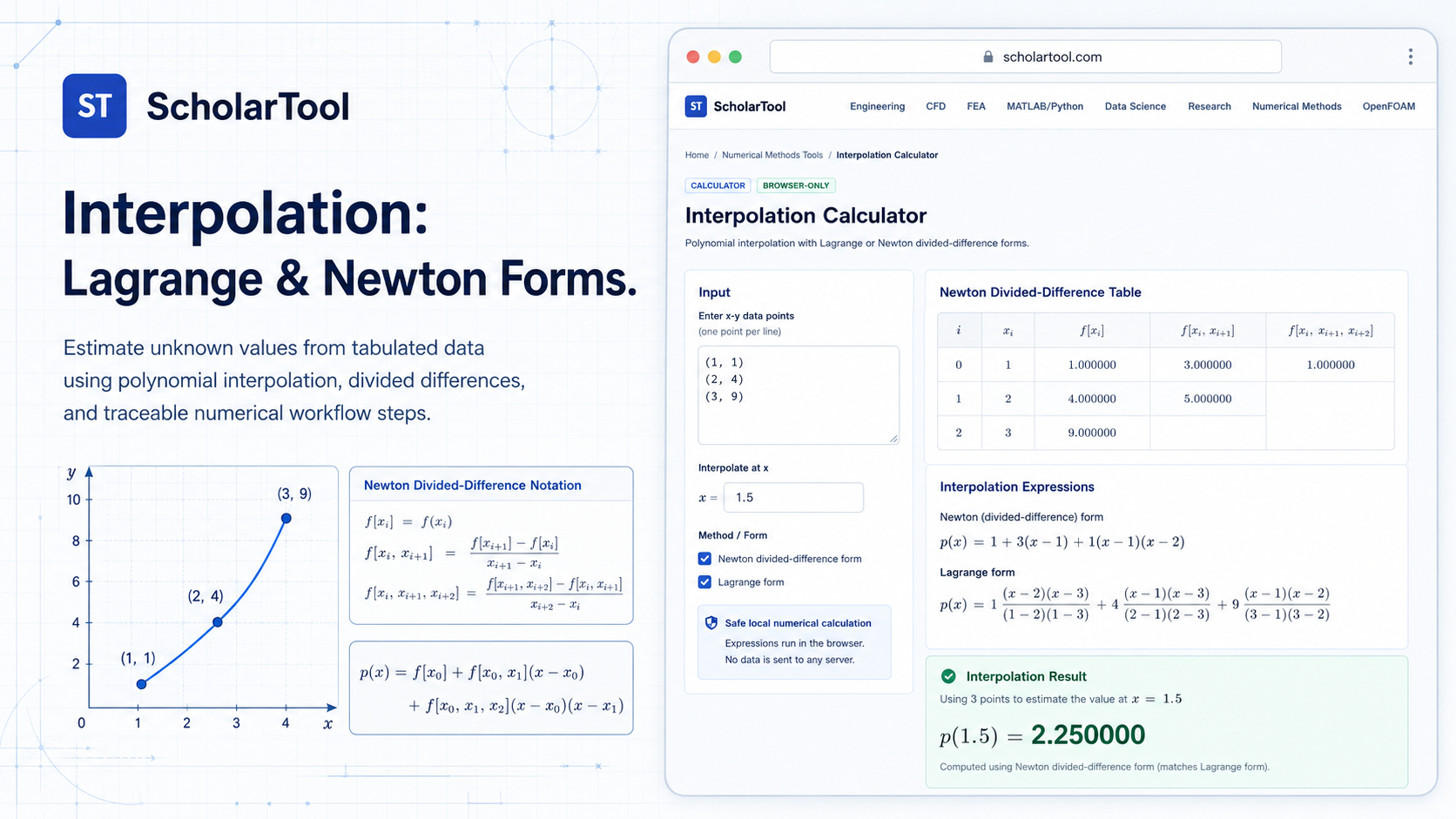
Interpolation Calculator: Lagrange & Newton Online Tool
When I am auditing a dataset from a material stress test or verifying a lookup table for a coordinate transformation, the “stumbling block” is rarely the data itself; it is the friction of the values I don’t have. As Joe Hoffman notes in Numerical Methods for Engineers and Scientists, in many problems, data is known only at discrete points rather than as a continuous function. To find values between these known coordinates, we must fit an approximating function a process known as interpolation.
What I find indispensable for these tasks is the Interpolation Calculator from ScholarTool. It is a deterministic, browser-local utility designed to construct polynomial interpolants using either the Lagrange or Newton divided-difference forms. Whether I am verifying a hand calculation for an assignment or grounding a preliminary engineering estimate in physical reality, this tool ensures my numerical assumptions are sound while keeping my proprietary research data entirely private.
What the Interpolation Calculator Helps You Do
The primary purpose of this tool is to provide a transparent, auditable path from a set of unique x-y pairs to a specific intermediate estimate. In technical terms, it fits a unique polynomial of degree $n$ or less that passes exactly through $n+1$ points.
I find the interface particularly helpful because it provides a “Comparative Perspective” on polynomial organization. As noted in the sources, while Lagrange and Newton forms describe the same polynomial, they organize the calculation differently. The Newton form is particularly useful because its coefficients are visible in a divided-difference table, allowing me to see the “math receipt” of the term-by-term construction. What I appreciate most is the “browser-only” architecture. Because the tool processes your points locally using TypeScript and a restricted math parser, your sensitive sensor data or internal research variables are never submitted to a third-party AI or remote server.
Inputs You Can Use
The interface is built with a configuration-first layout that ensures your data is valid before the calculator attempts to fit a polynomial.
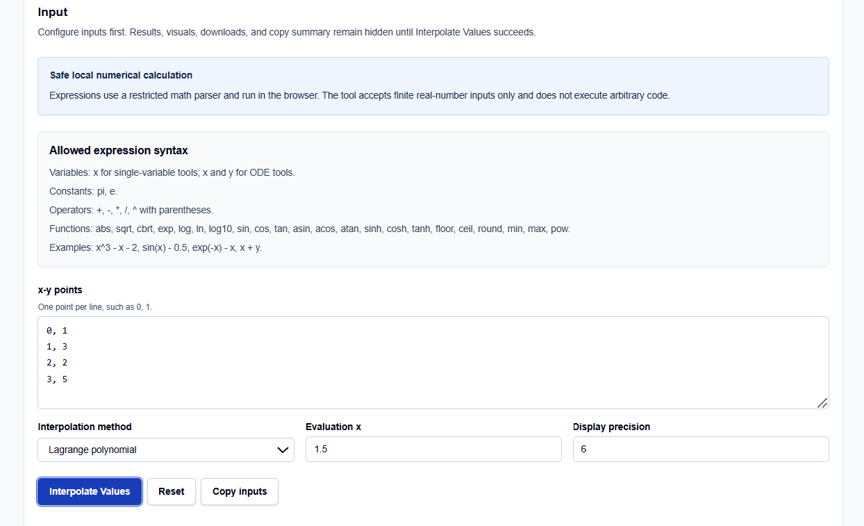
Data Points and Method Selection
I start by entering my x-y points, one pair per line (e.g., 0, 1 followed by 1, 3). You then select the Interpolation method: Lagrange polynomial or Newton divided differences. For Python or MATLAB practitioners, this choice is vital; as Chapra and Canale observe, the Lagrange version is often used when the order is known a priori, while Newton is better for sequential term development.
Evaluation and Precision
You define the Evaluation x the specific point where you need the interpolated value. You also have direct control over the Display precision, which dictates how many significant digits appear in the results. It is important to note that internal calculations maintain standard double-precision floating-point arithmetic for accuracy, even if the display is rounded.
How I Use the Tool
My typical workflow begins when a simulation log provides a series of discrete nodes, and I need a value between them for a documentation audit. I open the Interpolation Calculator and enter my tabulated data.
Once I have entered the points and the evaluation x, I click Interpolate Values. I find it useful that the results, visuals, and copy summaries remain hidden until this explicit action succeeds, preventing me from acting on stale or default data. I then review the Newton divided-difference coefficients (if selected) or the basis evaluations for the Lagrange form. If I need to test a different evaluation point, I rerun the calculation, knowing that the tool treats my inputs as plain text and processes them entirely within the page state.
Understanding the Results
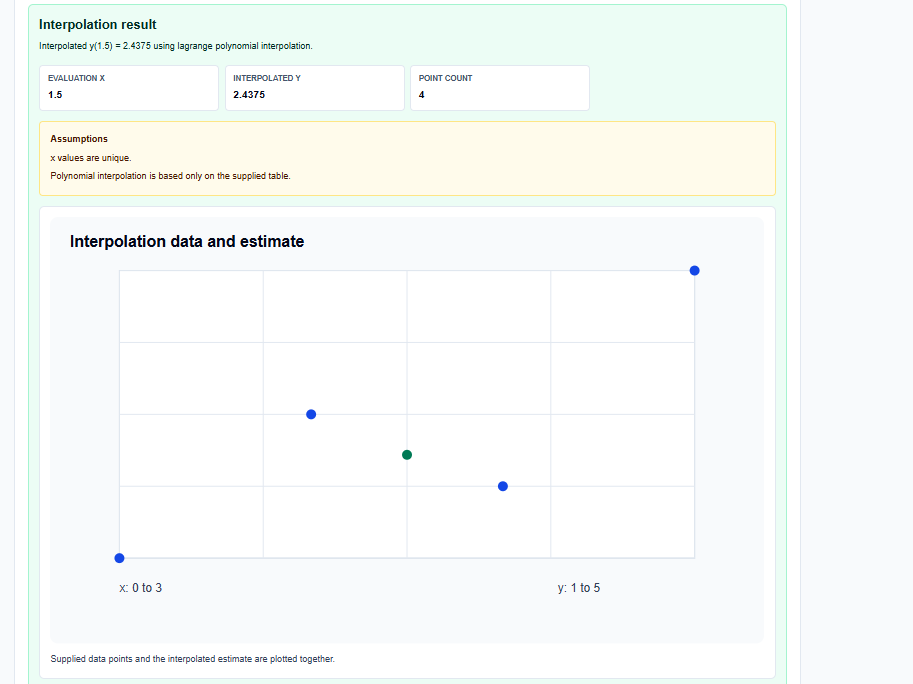
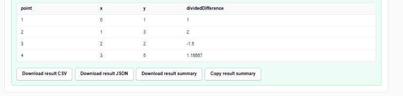
The result section provides the Main estimate first, followed by the Iteration history. For a professional audit, I focus on:
- Residual Checks: Verifies the quality of the fit at the input points.
- Divided-Difference Table: For Newton interpolation, this provides the coefficients $c_i$ used in the polynomial.
- Extrapolation Warnings: If my evaluation x falls outside the min/max range of my data, the tool issues an explicit warning, reminding me that extrapolation is less reliable than interpolation.
- Result-Driven Visual: The plot helps me detect if high-degree input is creating oscillatory behavior, a common risk with large point sets.
A Practical Example: Three-Point Interpolation
Suppose I have three points from a material test: (0, 1), (1, 3), and (2, 2). I need the value at x = 1.5. I enter these into the calculator and select “Newton divided differences.”
The Interpolation Calculator generates the divided differences and evaluates the polynomial. Because x = 1.5 is inside the supplied range, the tool identifies this as interpolation. The final result is a weighted sum of the data y-values, providing an exact point on the unique quadratic curve passing through those three nodes.
Mistakes I Would Avoid
One common pitfall is repeating x values. Polynomial interpolation mathematically requires unique x coordinates; entering the same x twice will lead to an invalid calculation.
Another mistake is using high-order polynomials on noisy data. As the sources warn, interpolation passes exactly through every point and can amplify noise, potentially creating physical behavior that doesn’t exist between the points. In such cases, I use the visual plot to ensure the curve is sensible for my engineering model.
Try the Free Interpolation Calculator
Before you spend another hour manually constructing divided-difference tables in your notebook, take a minute to generate a transparent calculation. It is the fastest way to ground your discrete data analysis in verified numerical logic while maintaining total data residency.
Try the Interpolation Calculator here.
To complete your numerical toolkit, you may also find the Numerical Integration Calculator or the Numerical Differentiation Calculator essential for your analysis workflow.
FAQ
1. What is the difference between Lagrange and Newton forms?
They represent the same unique polynomial but organize the calculation differently. The Newton form is advantageous for showing divided-difference coefficients in a table.
2. Can x values repeat in the dataset?
No. Polynomial interpolation requires unique x values to define a valid function.
3. Does the Interpolation Calculator run automatically while I type? No. To protect privacy and processing resources, results, visuals, and copy summaries remain hidden until you click the explicit “Interpolate Values” button.