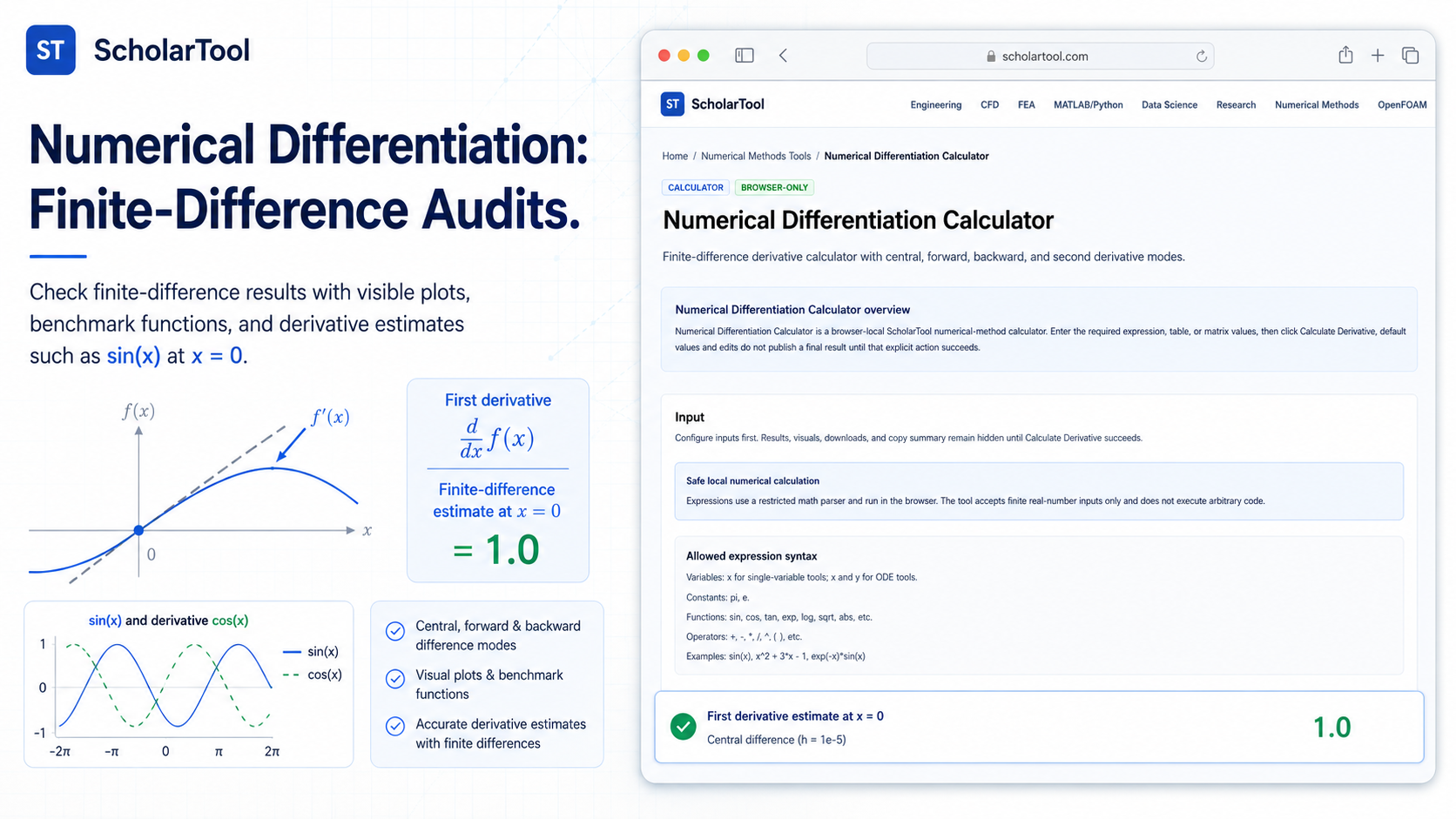
Numerical Differentiation Calculator: Finite-Difference Tool
When I am auditing a fluid dynamics simulation or characterizing the rate of change in a material stress test, the “stumbling block” is frequently a derivative that cannot be solved through simple symbolic rules. As Joe Hoffman notes in Numerical Methods for Engineers and Scientists, numerical differentiation is essential when a function is too complicated for manual calculus or when data is available only at discrete points. However, as any practitioner knows, it is also an inherently sensitive process small errors in data can lead to significant errors in the derivative.
What I find indispensable for these transitions is the Numerical Differentiation Calculator from ScholarTool. It is a deterministic, browser-local utility designed to evaluate finite-difference formulas. Whether I am verifying a hand calculation for an assignment or grounding a preliminary engineering estimate in physical reality, this tool ensures my numerical assumptions are sound while keeping my proprietary research data entirely private.
What the Numerical Differentiation Calculator Helps You Do
The primary purpose of this tool is to provide a transparent, auditable path from a mathematical expression or a table of values to a specific derivative estimate. In technical terms, it replaces exact calculus with approximating polynomials typically derived from Taylor series expansions to estimate the slope or curvature of a function at a specific point.
I find the interface particularly helpful because it prioritizes data residency. Unlike “black-box” solvers that upload your formulas to a remote AI server, this tool processes everything locally in your browser using TypeScript. This means your sensitive physics models or proprietary sensor data never leave your machine. It also avoids the risks of arbitrary code execution by utilizing a restricted math parser that accepts standard mathematical syntax but does not run scripts.
Inputs You Can Use
The interface is built with a configuration-first layout that ensures your setup is valid before results are generated.
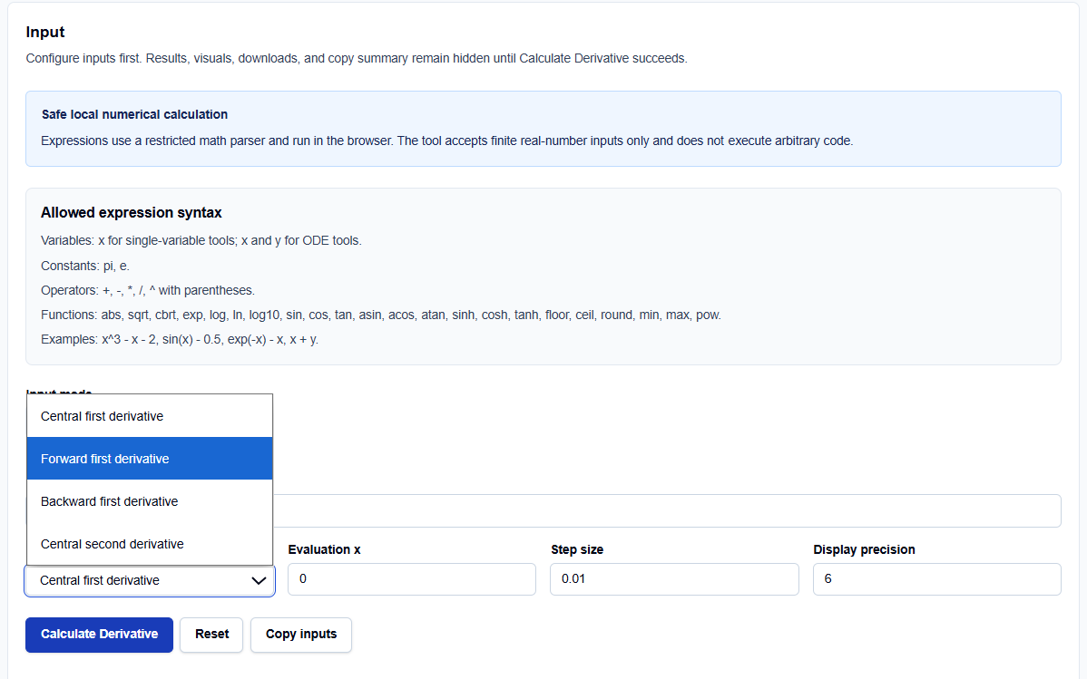
Input Modes and Syntax
You can toggle between Expression and Table modes. In Expression mode, you enter a function using the variable $x$. I find the support for a robust library of functions including exp, log, and full trigonometry essential for handling the transcendental equations common in engineering. In Table mode, you can paste x-y pairs directly from a spreadsheet, allowing the tool to evaluate slopes from neighboring data points.
Difference Methods and Controls
The tool supports four primary modes: Central first derivative, Forward first derivative, Backward first derivative, and Central second derivative. You specify the Evaluation x and the Step size (h). I always pay close attention to $h$; for a smooth function, a smaller $h$ generally reduces truncation error, but if $h$ is too small, it can amplify floating-point roundoff or noise in the data.
How I Use the Tool
My typical workflow begins when I have a complex function or a discrete dataset that needs a quick rate-of-change check. I open the Numerical Differentiation Calculator.
If I am using an expression, I enter the function and set the evaluation point. Once I have configured the step size and chosen a display precision, I click Calculate Derivative. I find it useful that the results, visuals, and copy summaries remain hidden until this explicit action succeeds, preventing me from acting on stale data. I then review the Sample values table to see exactly which points the tool evaluated to reach its estimate. If I am unsure of the stability, I rerun the tool with slightly different $h$ values to check for convergence.
A Comparative Perspective: Choosing Your Method
From a professional perspective, selecting a finite-difference scheme involves a trade-off between accuracy and data availability:
- Central Differences: I prefer these for most audits. As noted in the sources, central differences are generally $O(h^2)$ accurate, meaning the error decreases quadratically with $h$.
- Forward and Backward Differences: These are $O(h)$ accurate. I use these when I am at the boundary of a dataset where central sampling is impossible (e.g., at the start or end of a time-series log).
- Second Derivative: The central second derivative mode is vital when I need to assess curvature or acceleration from position data.
Understanding the Results
The result section provides the Main estimate first, followed by the Iteration/Sample history. For a professional audit, I focus on the secondary outputs:
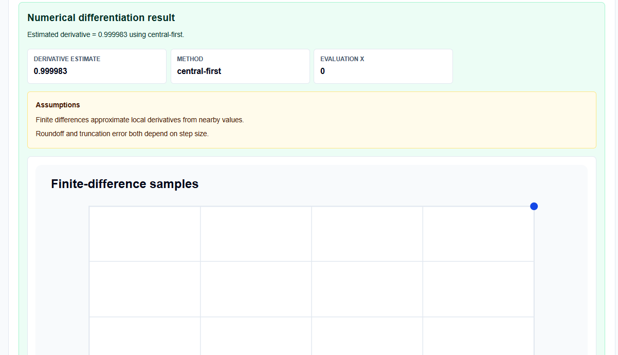
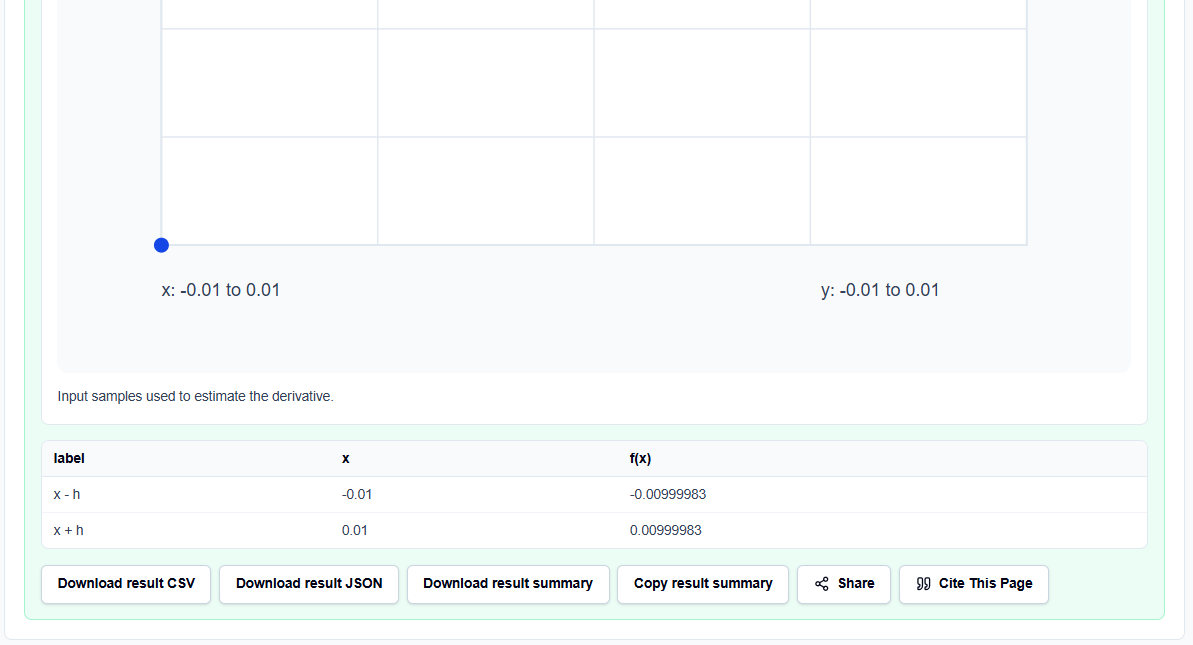
- Intermediate Sample Table: This reports the specific $x$ and $y$ values used in the formula, acting as a “math receipt” for my documentation.
- Interpretation Block: The tool identifies if the calculated values are consistent with the expected behavior of the entered model.
- Result-Driven Visual: This plot is vital for identifying if I have accidentally sampled near a singularity or if the function is oscillating too rapidly for the chosen step size.
A Practical Example: Differentiating a Sine Wave
Suppose I need to find the slope of $f(x) = \sin(x)$ at $x = 0$. I enter sin(x) as the expression, set $x = 0$, and use a step size $h = 0.01$. I select the Central first derivative method.
The Numerical Differentiation Calculator returns an estimate of 1.0 (or very near it, depending on the chosen precision). This benchmark allows me to verify the calculator’s logic against the known analytical derivative $\cos(0) = 1$ before I apply it to more complex research equations.
Mistakes I Would Avoid
One common pitfall is choosing h without checking sensitivity. As the tool’s common mistakes section warns, you should always rerun the calculation with nearby step sizes to ensure the result is stable.
Another mistake is using central table differences at an endpoint. If your data ends at $x=10$, a central difference requires a point at $x > 10$. In these cases, I always switch to the Backward first derivative mode to ensure the calculation remains valid within the data range.
Try the Free Numerical Differentiation Calculator
Before you spend another hour manually unrolling Taylor series expansions in your notebook, take a minute to generate a transparent finite-difference estimate. It is the fastest way to ground your rate-of-change calculations in verified numerical logic while maintaining total data residency.
Try the Numerical Differentiation Calculator here.
To complete your numerical toolkit, you may also find the Numerical Integration Calculator or the Interpolation Calculator essential for your analysis workflow.
FAQ
1. What step size (h) should I choose?
Generally, start with a small value like 0.01 or 0.001. You should always rerun the calculator with nearby step sizes to verify that the result remains stable and is not being corrupted by floating-point roundoff.
2. Can I use this for data I copied from Excel?
Yes. Use the Table mode and paste your x-y pairs, one per line. Ensure that your evaluation $x$ matches a point in your table and that you have the neighboring points required for your selected formula (e.g., central differences need points on both sides).
3. Does this tool perform symbolic differentiation?
No. This is a numerical tool that estimates derivatives using finite-difference formulas. It is designed for cases where an analytical solution is unavailable or where you are working with discrete tabular data.